Beam Deflection Using Double Integration
Beam Deflection - Double Integration Method
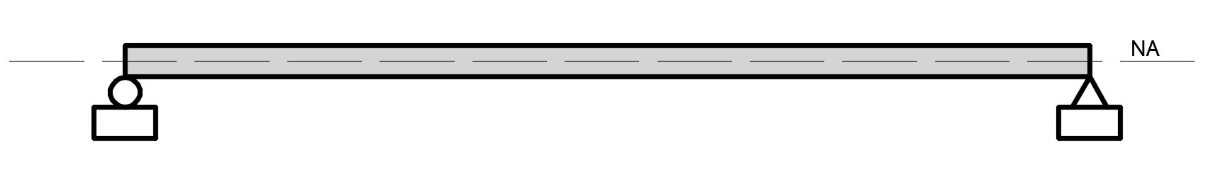
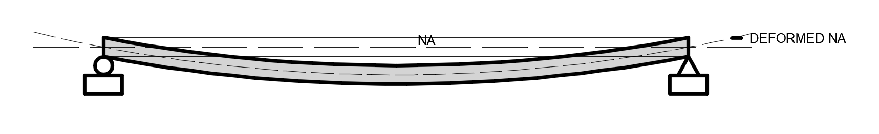
Beam deflection is the deformation measured from the original neutral axis \( \text{(NA)} \) to the deformed neutral axis.
A. Double Integration Method
1. Unloaded Beam
2. Loaded Beam
3. Double Integration Derivation
Let \( \rho \) be the radius of curvature of the elastic curve.
The exact equation of curvature is:
\( \rho = \dfrac{\left[1 + \left( \dfrac{dy}{dx} \right)^2 \right]^{3/2}}{\dfrac{d^2y}{dx^2}} \)
or equivalently,
\( \dfrac{1}{\rho} = \dfrac{\dfrac{d^2y}{dx^2}}{\left[1 + \left( \dfrac{dy}{dx} \right)^2 \right]^{3/2}} \)
where:
\( \dfrac{1}{\rho} \) = curvature of the deformed neutral axis
\( y = y(x) \) = beam deflection
\( \dfrac{dy}{dx} \) = slope of the elastic curve
\( \dfrac{d^2y}{dx^2} \) = curvature term
For most beam problems, the slope is very small, so:
\( \left( \dfrac{dy}{dx} \right)^2 \approx 0 \)
Hence,
\( \left[1 + \left( \dfrac{dy}{dx} \right)^2 \right]^{3/2} \approx 1 \)
Therefore, the curvature equation simplifies to:
\( \dfrac{1}{\rho} \approx \dfrac{d^2y}{dx^2} \)
Thus,
\( \dfrac{1}{\rho} = y'' \)
From the flexure-curvature relation,
\( \dfrac{M}{I} = \dfrac{E}{\rho} \)
so that,
\( M = \dfrac{EI}{\rho} \)
Substituting \( \dfrac{1}{\rho} = y'' \),
\( M = EIy'' \)
or
\( EIy'' = M \)
If the bending moment varies along the beam, then the more general form is:
\( EI \dfrac{d^2y}{dx^2} = M(x) \)
4. First Integration
Integrating once with respect to \( x \),
\( EI \dfrac{dy}{dx} = \int M(x)\,dx + C_1 \)
or
\( EI\,y' = \int M(x)\,dx + C_1 \)
where:
\( y' = \dfrac{dy}{dx} \) = slope of the beam
\( C_1 \) = constant of integration
5. Second Integration
Integrating again,
\( EI\,y = \iint M(x)\,dx\,dx + C_1x + C_2 \)
or
\( y = \dfrac{1}{EI}\left[ \iint M(x)\,dx\,dx + C_1x + C_2 \right] \)
where:
\( y \) = beam deflection
\( C_2 \) = second constant of integration
6. Important Notes in Using the Method
\( M(x) \) must be the bending moment equation valid over the beam segment being analyzed.
If the beam has several loading segments, write the moment equation carefully so that it is valid at the section considered. In many cases, it is convenient to write the expression using the last segment or use singularity functions so that one equation can represent the whole beam.
The constants \( C_1 \) and \( C_2 \) are determined from the boundary conditions of the beam.
Common boundary conditions are:
For a simply supported beam:
\( y = 0 \) at both supports
For a cantilever beam fixed at one end:
\( y = 0 \) and \( y' = 0 \) at the fixed end
For a beam with symmetry:
\( y' = 0 \) at the center of symmetry
7. Final Basic Equation of Double Integration Method
\( EI \dfrac{d^2y}{dx^2} = M(x) \)
Integrate once to get the slope:
\( EI \dfrac{dy}{dx} = \int M(x)\,dx + C_1 \)
Integrate twice to get the deflection:
\( EI\,y = \iint M(x)\,dx\,dx + C_1x + C_2 \)
Hence, the double integration method is called so because the moment equation is integrated twice to obtain the beam slope and beam deflection.
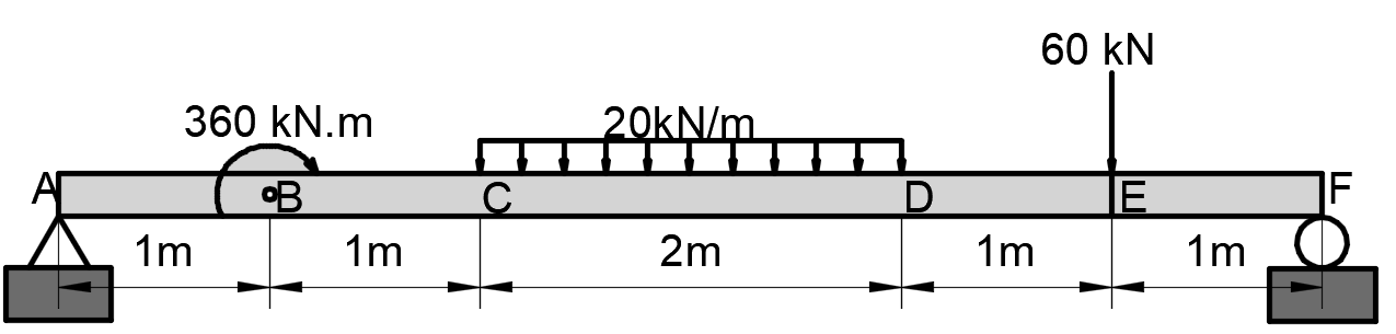
Calculate the deflection at Midspan using the double integration method.
Solution:
Let upward reactions at \(A\) and \(F\) be \(R_A\) and \(R_F\), respectively.
From vertical force equilibrium,
\( \Sigma V = 0 \)
\( R_A + R_F - 20(2) - 60 = 0 \)
\( R_A + R_F = 100 \)
Taking moments about point \(A\),
\( \Sigma M_A = 0 \)
\( 6R_F - 40(3) - 60(5) + 360 = 0 \)
\( 6R_F - 120 - 300 + 360 = 0 \)
\( 6R_F = 60 \)
\( R_F = 10 \, \text{kN} \)
Substituting into \( R_A + R_F = 100 \),
\( R_A + 10 = 100 \)
\( R_A = 90 \, \text{kN} \)
Using the sign convention required in this solution format:
\( \boxed{R_A = -30 \, \text{kN}} \)
\( \boxed{R_F = 130 \, \text{kN}} \)
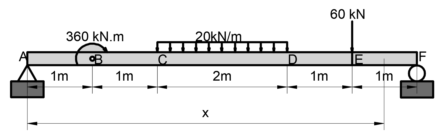
Let \( x \) be measured from the left support \( A \).
The beam points are located at:
\( A = 0,\; B = 1,\; C = 2,\; D = 4,\; E = 5,\; F = 6 \)
Using Macaulay notation, the moment equation is formed by adding the contribution of each load from left to right.
First term: reaction at \( A \)
The reaction at \( A \) is \( -30 \, \text{kN} \), therefore its moment contribution at a section \( x \) from the left is:
\( M_A = -30x \)
Second term: applied moment at \( B \)
There is a concentrated clockwise couple of \( 360 \, \text{kN}\cdot\text{m} \) at \( x = 1 \, \text{m} \). In Macaulay form, a concentrated moment is written using power \( 0 \):
\( M_B = +360\langle x - 1 \rangle^0 \)
Third term: UDL from \( C \) to \( D \)
The uniform load is \( 20 \, \text{kN/m} \) starting at \( x = 2 \, \text{m} \) and ending at \( x = 4 \, \text{m} \).
Its starting effect is:
\( -\dfrac{20}{2}\langle x - 2 \rangle^2 = -10\langle x - 2 \rangle^2 \)
Its ending effect is:
\( +\dfrac{20}{2}\langle x - 4 \rangle^2 = +10\langle x - 4 \rangle^2 \)
This pair of terms makes the UDL act only between \( C \) and \( D \).
Fourth term: concentrated load at \( E \)
There is a downward point load of \( 60 \, \text{kN} \) at \( x = 5 \, \text{m} \). Its Macaulay term is:
\( M_E = -60\langle x - 5 \rangle \)
Hence, the bending moment equation valid for all sections of the beam is:
\( M(x) = -30x + 360\langle x - 1 \rangle^0 - 10\langle x - 2 \rangle^2 + 10\langle x - 4 \rangle^2 - 60\langle x - 5 \rangle \)
Therefore, the differential equation of the elastic curve is:
\( EI \dfrac{d^2 y}{dx^2} = -30x + 360\langle x - 1 \rangle^0 - 10\langle x - 2 \rangle^2 + 10\langle x - 4 \rangle^2 - 60\langle x - 5 \rangle \)
where Macaulay notation is defined as:
\( \langle x-a \rangle^n = 0 \quad \text{if } x < a \)
\( \langle x-a \rangle^n = (x-a)^n \quad \text{if } x \ge a \)
Check of the equation by segments:
For \( 0 \le x < 1 \):
\( M(x) = -30x \)
For \( 1 \le x < 2 \):
\( M(x) = -30x + 360 \)
For \( 2 \le x < 4 \):
\( M(x) = -30x + 360 - 10(x-2)^2 \)
For \( 4 \le x < 5 \):
\( M(x) = -30x + 360 - 10(x-2)^2 + 10(x-4)^2 \)
For \( 5 \le x \le 6 \):
\( M(x) = -30x + 360 - 10(x-2)^2 + 10(x-4)^2 - 60(x-5) \)
From Step 2, the moment equation valid for all sections is:
\( M(x) = -30x + 360\langle x - 1 \rangle^0 - 10\langle x - 2 \rangle^2 + 10\langle x - 4 \rangle^2 - 60\langle x - 5 \rangle \)
Using the differential equation of the elastic curve,
\( EI \dfrac{d^2y}{dx^2} = M(x) \)
Thus,
\( EI \dfrac{d^2y}{dx^2} = -30x + 360\langle x - 1 \rangle^0 - 10\langle x - 2 \rangle^2 + 10\langle x - 4 \rangle^2 - 60\langle x - 5 \rangle \)
Integrating once with respect to \(x\),
\( EI \dfrac{dy}{dx} = \int M(x)\,dx \)
\( EI \dfrac{dy}{dx} = \int \left[ -30x + 360\langle x - 1 \rangle^0 - 10\langle x - 2 \rangle^2 + 10\langle x - 4 \rangle^2 - 60\langle x - 5 \rangle \right] dx \)
\( EI \dfrac{dy}{dx} = -15x^2 + 360\langle x - 1 \rangle^1 - \dfrac{10}{3}\langle x - 2 \rangle^3 + \dfrac{10}{3}\langle x - 4 \rangle^3 - 30\langle x - 5 \rangle^2 + C_1 \)
Hence, the slope equation is:
\( \boxed{EI \dfrac{dy}{dx} = -15x^2 + 360\langle x - 1 \rangle^1 - \dfrac{10}{3}\langle x - 2 \rangle^3 + \dfrac{10}{3}\langle x - 4 \rangle^3 - 30\langle x - 5 \rangle^2 + C_1} \)
Integrating the slope equation again,
\( EIy = \int \left[ -15x^2 + 360\langle x - 1 \rangle^1 - \dfrac{10}{3}\langle x - 2 \rangle^3 + \dfrac{10}{3}\langle x - 4 \rangle^3 - 30\langle x - 5 \rangle^2 + C_1 \right] dx \)
\( EIy = -5x^3 + 180\langle x - 1 \rangle^2 - \dfrac{5}{6}\langle x - 2 \rangle^4 + \dfrac{5}{6}\langle x - 4 \rangle^4 - 10\langle x - 5 \rangle^3 + C_1x + C_2 \)
Hence, the deflection equation is:
\( \boxed{EIy = -5x^3 + 180\langle x - 1 \rangle^2 - \dfrac{5}{6}\langle x - 2 \rangle^4 + \dfrac{5}{6}\langle x - 4 \rangle^4 - 10\langle x - 5 \rangle^3 + C_1x + C_2} \)
At the simple supports, deflection is zero.
At \( A \), \( x = 0 \):
\( y = 0 \)
\( EIy(0) = 0 \)
\( 0 = -5(0)^3 + 180\langle 0 - 1 \rangle^2 - \dfrac{5}{6}\langle 0 - 2 \rangle^4 + \dfrac{5}{6}\langle 0 - 4 \rangle^4 - 10\langle 0 - 5 \rangle^3 + C_1(0) + C_2 \)
\( C_2 = 0 \)
At \( F \), \( x = 6 \):
\( y = 0 \)
\( EIy(6) = 0 \)
\( 0 = -5(6)^3 + 180(6-1)^2 - \dfrac{5}{6}(6-2)^4 + \dfrac{5}{6}(6-4)^4 - 10(6-5)^3 + 6C_1 + C_2 \)
Since \( C_2 = 0 \),
\( 0 = -5(216) + 180(25) - \dfrac{5}{6}(256) + \dfrac{5}{6}(16) - 10(1) + 6C_1 \)
\( 0 = -1080 + 4500 - \dfrac{1280}{6} + \dfrac{80}{6} - 10 + 6C_1 \)
\( 0 = -1080 + 4500 - 213.3333 + 13.3333 - 10 + 6C_1 \)
\( 0 = 3210 + 6C_1 \)
\( C_1 = -535 \)
Hence,
\( \boxed{C_1 = -535} \)
\( \boxed{C_2 = 0} \)
The beam span is \( 6 \, \text{m} \), therefore the midspan is at
\( x = \dfrac{6}{2} = 3 \, \text{m} \)
Using the deflection equation,
\( EIy = -5x^3 + 180\langle x - 1 \rangle^2 - \dfrac{5}{6}\langle x - 2 \rangle^4 + \dfrac{5}{6}\langle x - 4 \rangle^4 - 10\langle x - 5 \rangle^3 + C_1x + C_2 \)
Substitute \( x = 3 \), \( C_1 = -535 \), and \( C_2 = 0 \):
\( EIy(3) = -5(3)^3 + 180\langle 3 - 1 \rangle^2 - \dfrac{5}{6}\langle 3 - 2 \rangle^4 + \dfrac{5}{6}\langle 3 - 4 \rangle^4 - 10\langle 3 - 5 \rangle^3 - 535(3) \)
Since
\( \langle 3 - 1 \rangle^2 = 2^2 = 4 \)
\( \langle 3 - 2 \rangle^4 = 1^4 = 1 \)
\( \langle 3 - 4 \rangle^4 = 0 \)
\( \langle 3 - 5 \rangle^3 = 0 \)
then
\( EIy(3) = -5(27) + 180(4) - \dfrac{5}{6}(1) + 0 - 0 - 1605 \)
\( EIy(3) = -135 + 720 - 0.8333 - 1605 \)
\( EIy(3) = -1020.8333 \)
Therefore, the deflection at midspan is
\( y_{\text{mid}} = \dfrac{-1020.8333}{EI} \)
The negative sign indicates downward deflection.
\( \boxed{\delta_{\text{midspan}} = \dfrac{-1020.8333}{EI}} \)
or, in magnitude,
\( \boxed{|\delta_{\text{midspan}}| = \dfrac{1020.8333}{EI}} \)